What is Indifference Curve?
An indifference curve is a graphical representation used in microeconomics to illustrate consumer preferences and choices. It shows different combinations of two goods or commodities that provide the same level of satisfaction or utility to a consumer. In other words, each point on an indifference curve represents a specific combination of the two goods that the consumer considers equally preferable.
Properties of Indifference Curves:
Following are the properties of indifference curves.
(1) They slope negatively or slope downwards from the left to the right. This is an important feature of indifference curves. The reason is obvious. For example- a consumer is confronted with various combinations of bananas and oranges- each combination giving him the same total satisfaction. Now, if the total satisfaction is to remain the same, the consumer must part with a diminishing number of bananas (downward movement) as he gets an increasing stock of oranges (rightward movement). The loss of satisfaction to the consumer on account of the downward movement must be made up by the gain through the rightward movement. As such, the indifference curve must slope downwards to the right.
We can also establish this conclusion if we are able to prove that an upward-slopping curve or a horizontal curve or a vertical curve is an impossibility. Just imagine an indifference curve that slopes upwards to the right. As the consumer moves upwards along this curve, he gets more and more of both commodities, say, bananas and oranges. His total satisfaction cannot, therefore, remain constant. It must increase as he moves up along the curve. He can no longer remain indifferent between two points on this curve. This would be obvious from Diagram (A).
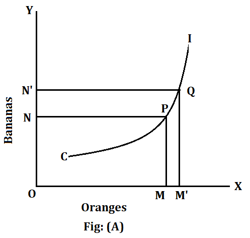
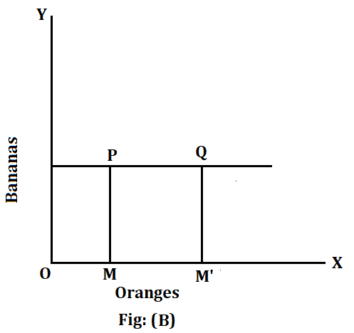
In this diagram, at point P, the consumer gets OM of oranges and ON of bananas. At Q, he gets OM’ of oranges and ON’ of bananas. Obviously, at Q he gets more of both commodities. Therefore, his total satisfaction is greater at Q than at P. How can he be indifferent between these two points? Curve IC cannot, therefore, be the indifference curve. The various points on an indifference curve yield the same total satisfaction to the consumer. The same argument applies to a curve that is horizontal or vertical. On such a curve, he gets the same quantity of one good but more and more of the other. Diagram (B) makes it clear: At point P, the consumer gest OM of oranges and ON of bananas. At Q, he obtains OM’ of oranges but the same ON quantity of bananas. In other words, he gets more of oranges at Q, though the quantity of bananas remains the same. Obviously, the consumer gets greater satisfaction at Q than at P. He cannot remain indifferent between these two points. He will prefer Q to P.
Likewise, a vertical curve cannot be an indifference curve. This would be obvious from Diagram (C).
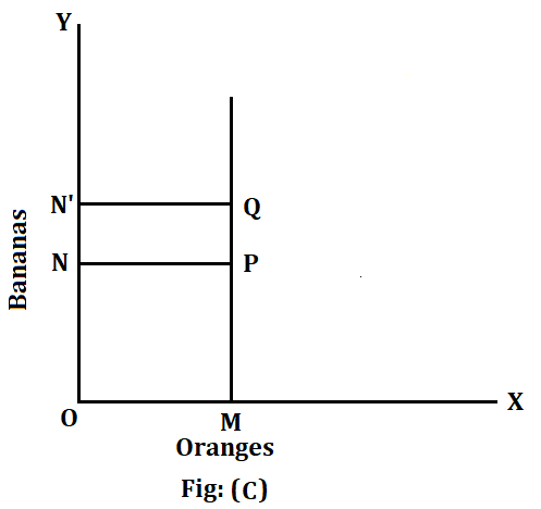
In this diagram at P, the consumer obtains OM of oranges and ON of bananas. At Q, he gets the same OM oranges, but ON’ of bananas. Obviously, he secures greater total satisfaction at Q than at P. He cannot, therefore, be indifferent between P and Q. We have thus proved that an indifference curve cannot slope upward to the right. Nor can it be horizontal or vertical. The only possibility, therefore, is that it must slope downwards to the right. The consumer will get additional supplies of oranges by sacrificing diminishing quantities of bananas.
(2) They are convex to the origin of axes. The second property of the indifference curves is that they are generally convex to the origin of the axes- the left-hand portion is normally steep while the right-hand portion is relatively flat. This property of the indifference curve is derived from the law of diminishing marginal rate of substitution. We have already seen that the marginal rate of substitution neither increases nor does it remain constant.
If the marginal rate of substitution had increased, the indifference curve would have been concave to the origin. If, on the other hand, the marginal rate of substitution had remained constant, the indifference curve would have been a diagonal straight line at a 45-degree angle. But, as we have seen, the marginal rate of substitution neither increases nor does it remain constant. The marginal rate of substitution, on the contrary, goes on diminishing. As such, the indifference curve has to be convex to the origin of axes. In terms of our example, the greater the number of oranges that are acquired, the smaller the number of bananas that will be substituted to maintain a given level of total satisfaction. In other words, an additional orange will progressively replace a smaller and smaller number of bananas. This will be obvious from Diagram (D).
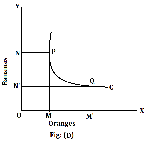
In this diagram, an increase of oranges from OM to OM’ is accompanied by a progressively diminishing number of bananas from ON to ON’. Thus a falling curve whose slope diminishes as we move to the right is bound to be convex to the origin of axes.
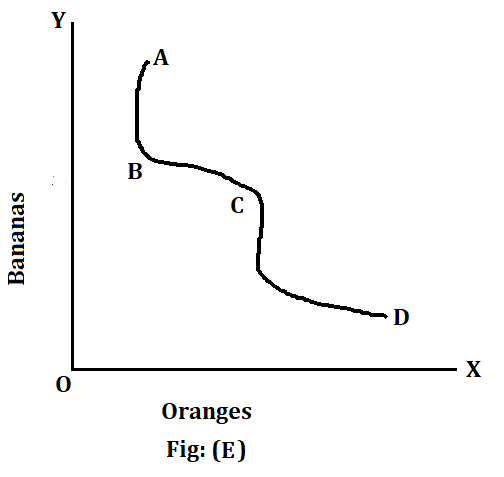
It should be remembered that concavity in an indifference curve occurs only if the marginal rate of substitution is increasing. Since an increasing marginal rate of substitution is not a normal phenomenon, the indifference curve is not likely to be concave to the origin of the axes. It is more likely to be convex rather than concave to the origin of the axes. This, however, does not imply that over limited ranges the indifference curve may not be concave. In other words, some ‘wobbles’ or ‘bumps of concavity’ could occur over some ranges of the indifference curve. An example of this kind of situation is given in the diagram (E). In this diagram, the indifference curve is convex from A to B, then becomes concave from B to C and once again becomes convex from C to D. From A to B, the marginal rate of substitution is declining. The consumer is prepared to surrender progressively fewer bananas to acquire extra oranges. So this part of the curve from A to B is convex. At point B, a sudden reversal takes place. The consumer now suddenly becomes prepared to part with an increasing number of bananas to obtain extra oranges. The marginal rate of substitution increases and the curve becomes concave. This continues until point C is reached when conditions again change and the consumer is now willing to part with fewer and fewer bananas for each extra orange. The marginal rate of substitution once again starts diminishing and the curve becomes convex to the origin. Thus, from A to B and from C to D the indifference curve displays a normal shape with a diminishing marginal rate of substitution in terms of banans. But the portion of the curve from B to C shows an abnormal shape with an increasing marginal rate of substitution between the two commodities.
It should, however, be pointed out that the consumer will never find himself in equilibrium while he remains on the concave range of the indifference curve. Since the marginal rate of substitution in terms of bananas is increasing, it will not pay him to go on surrendering more and more of them against oranges. Ultimately the indifference curve will become convex again. The ‘bumps of concavity’ on the indifference curve are then a purely temporary phenomenon. We are not, therefore, wrong if we assume that indifference curves are always conex to the origin.
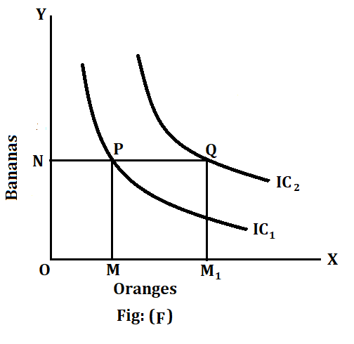
(3) Every indifference curve to the right represents a higher level of satisfaction than that of the preceding one. To show this, let us take two indifference curves IC1 and IC2, IC2 lying to the right of IC1 [see Diagram (F)]. At point P, the consumer gets OM of oranges and ON of bananas. At point Q, though the number of bananas remains the same i.e., ON, yet the number of oranges increases from OM to OM1. The total satisfaction of the consumer is, therefore, bound to be greater at Q than at P. Hence Q represents a more valued and preferred combination of oranges and bananas than P. As all the points on one indifference curve represent equal satisfaction, therefore, every point on IC, represents a combination preferred to that represented by any point on IC1. An indifference curve to the right represents a preferred position and therefore a consumer would always try to move on the indifference map as much to the right as possible.
(4) No two indifference curves can intersect each other. The fourth property of indifference curves is that no two indifference curves can ever cut each other.
The reality of this characteristic can be clearly seen in Diagram (G) where two indifference curves have been shown as cutting each other. Since point A is on the indifference curve IC2, it represents a higher level of satisfaction to the consumer than at point B which is located on the lower indifference curve IC1. Point C, however, lies on both curves. This means that two levels of satisfaction, A and B which are by definition unequal, manage to become equal at point C. This is clearly impossible. Indifference curves can never intersect each other.

(5) Indifference curves need not necessarily be parallel to each other. This is due to two reasons. Firstly, the indifference curves are not based on the cardinal measurability of utility. Secondly, the rate of substitution between the two commodities need not be the same in all the indifference schedules. It is, therefore, not necessary that the indifference curves should be parallel to each other. In fact, they can be drawn in any manner one likes-parallel or unparallel to each other.



Comments (No)